Structuredness as a Measure of the Complexity of the Structure and the Role of Post-Dissipative Structures and Ratchet Processes in Evolution

The notion of complexity was originally a qualitative concept. But about half a century ago, Ray Solomonoff ⁹, Andrey Kolmogorov ¹⁰ and Gregory Chaitin ¹¹, using an algorithmic approach, proposed a rigorous mathematical definition of complexity. All three authors independently defined the algorithmic or descriptive complexity K(x) of the final object x as the length of the shortest computer program, which prints a complete, but not redundant (i.e., minimal), binary description of x, and then halts.

If D is a set of d_x as all possible descriptions of x, L is the equipotent set of lengths l_x of all descriptions d_x and l_pr is the binary length of the program mentioned above, the algorithmic complexity K(x), often called Kolmogorov complexity, equals to:

K(x) = l_pr + Min(l_x) ……..(2)

or, if x is not binary, but some other description that uses n symbols, then:

K(x) = l_pr + Min(1nk=1npklog pk) ……..(3)

To estimate K(x) for a material system, one must first describe it. In other words, you need to create a mathematical model of the system, then implement this model as a computer program and finally write another program that prints the first program and then halts. Of course, any model is not a complete description of the system and cannot avoid some redundancies. But improvements in the model bring the calculated complexity estimates closer to its exact value. And this exact value, as was shown earlier ¹, monotonously increases with the growth of information and entropy.

Although the algorithmic complexity is probably the only one that is determined strictly and unambiguously, there are many other, broader but less rigorous interpretations of this concept. Some of them consider the states of maximal entropy and randomization, i.e., chaos, as simple, which also looks quite logical. At the same time, the states of minimal entropy and, respectively, maximum order are considered as simple ones, too. Accordingly, the maximum complexity in this approach lies somewhere between order and chaos ^{12, 13}. Such an interpretation of complexity is consistent with its intuitive understanding and, at the same time, clearly contradicts the algorithmic definition.

However, if we consider this approach more deeply, it can be noted that we are talking about the complexity of the structure, not of the complexity itself. Indeed, the maximum order has no structure, or at least its structure is extremely simple. At the same time, a chaotic conglomerate of any objects, which also does not look like a structure, cannot be considered as something simple. Thus, it would be better not to confuse this concept with complexity as such and to emphasize each time that this is precisely the complexity of the structure and nothing more. This would eliminate the contradiction of this parameter with the algorithmic complexity.

There is another significant difference between the algorithmic complexity and the complexity of the structure. If the former has a clear mathematical definition and can be calculated, at least in principle, the latter is determined to a large extent, qualitatively or even intuitively. Numerous measures of complexity, such as “logical depth” ¹⁴, “sophistication” ¹⁵, “stochastic complexity” ¹⁶ and many others that are quite quantitative, mainly develop the algorithmic complexity in one direction or another, and not to measure the structural one.

Meanwhile, we will not be able to advance further on the path to understanding the general role of the laws of nature in the process of complification without quantifying the structural complexity and its connection with algorithmic complexity, information, and entropy. In the next section, I will offer such a measure in two – intensive and extensive - variants and illustrate its behavior with examples of some model and real systems.

It makes sense to start with an intensive measure. It is obvious that such measure should depend on the detailing of the structure, its diversity and intricacy. The most commonly used measure of this diversity is Shannon entropy H (see formula 1 above). However, H is obviously an extensive parameter, and the more, the more number of elements i. To avoid this extensiveness, I normalized H to the interval (0, 1):

h_r = H_r /H_max, ……..(4)

where h_ris normalized Shannon entropy, H_r is the entropy of rth state and H_max is the maximum possible entropy when each p_i equals one to another, i.e.

H_max = ̶ K N (1/N log(1/N)) = ̶ Klog(1/ N) = K log N, ……... (5)

where N is totalnumber of elements: 1, 2, … i, … N.

Now, if to substitute formula 1 and 5 into 4, h_requals to

h_r = ̶ K Σp_ir log p_ir) / (K log N) = ̶ Σp_ir log p_ir) / log N. ……..(6)

Such normalized entropy was already used in various fields (see, for example, ¹⁷ or ¹⁸) but this measure is not exactly that we need. The fact is that the normalized entropy measures the general complexity not structural, and equals to 1 for a chaotic state in which there are no structures. What we really need is a function that is 0 when its argument is either 0 or 1 and have one maximum in between. In 1948, Clod Shannon ¹⁹ proved the theorem according to which there is one and only one function corresponding to this condition. And this function is H from formula 1.

If we apply the function H to h_rfrom formula 6, we obtain the intensive measure of structural complexity that we are looking for. I would suggest to call this measure in general structuredness and designate it by Greek letter Δ from Δομή which in Greek means “structuredness”. Wherein, its lowercase – δ – could be used for the intensive measure while its uppercase – Δ – for the extensive one. Accordingly, the intensive measure of structuredness, i.e., normalized structuredness, will be equal to

δ_r = ̶ h_r log h_r ̶ (1 ̶ h_r) log (1 ̶ h_r), ……..(7)

where constant K_δ(which generally is not equal to K in formulas 1, 5 and 6) was set to 1 for simplicity. And if we replace h_r in formula 7 with its expression from formula 6, we get:

Figure 1demonstrates how the normalized structuredness δ depends on the normalized entropy. The maximum value on this curve is 1 in units of the constant K_δ. This maximum corresponds to a structure with a maximum structural complexity, which is achieved when the total algorithmic complexity of the system is equal to half of the maximum possible, which is the simplest ideal case.

Figure 1.Dependence of the normalized structuredness (δ) measured in units of constant Kδ on the normalized entropy (h), by the formula 7. 

Let me illustrate the behavior of such structuredness on the interval (0,1) by the example of a model algorithmic system. This system reaches the maximum of its algorithmic complexity when its binary description is completely stochastic and chaotic, like this:

0 1 0 0 0 1 1 1 0 1 1 0 0 1 0 0 1 0 0 0 0 1 1 1 0 0 1 1 1 0 1 0 0 1 1 0 0 0 0 1 0 1 1 0 1 0 0 1 1 1 1

Accordingly, h for such description is 1 and δ = 0. If, on the contrary, the system is completely degenerate, ordered and as simple as possible:

0 0 0 0 0 0 0 0 0 0 0 0 0 0 0 0 0 0 0 0 0 0 0 0 0 0 0 0 0 0 0 0 0 0 0 0 0 0 0 0 0 0 0 0 0 0 0 0 0 0 0

or

1 1 1 1 1 1 1 1 1 1 1 1 1 1 1 1 1 1 1 1 1 1 1 1 1 1 1 1 1 1 1 1 1 1 1 1 1 1 1 1 1 1 1 1 1 1 1 1 1 1 1

it has h = 0, but, according to formula 7 and the curve in Figure 1, its δ = 0, too.

Thus, there are two possible directions for increasing of normalized structuredness: from chaos (by ordering) and from order (by disordering). In the first case, an increase in structuredness is accompanied by a decrease in normalized entropy and, accordingly, of algorithmic complexity. In the second one, the increasing in structuredness goes in parallel with the increasing of the algorithmic complexity.

The first direction is manifested in the appearance of small local structures among the general chaos. The following binary description can be an example of the first steps in this direction from chaos to structuredness:

1 1 0 0 0 0 1 1 0 1 1 0 0 0 1 1 0 1 1 0 0 1 1 0 1 1 0 0 0 0 1 1 0 1 1 0 0 1 1 0 0 0 1 0 0 1 1 0 1 1 0

Here we see the simplest structure (1 1) which appears stochastically among the zeros. Such local structures can become more and more organized, which reduces the algorithmic complexity and increases the structuredness.

The second direction starts from the simplest global structures that are only slightly more complicated than fully ordered or degenerate (see above) due to rare defects. Here are a couple examples of relevant binary descriptions:

1 0 0 0 0 0 0 0 0 0 0 0 0 0 0 0 0 0 0 0 0 0 0 0 0 0 0 0 0 0 0 0 0 0 0 0 0 0 0 0 0 0 0 0 0 0 0 0 0 0 0

and

1 1 1 1 1 1 1 1 1 1 1 1 1 1 1 1 1 1 1 1 1 1 1 1 0 1 1 1 1 1 1 1 1 1 1 1 1 1 1 1 1 1 1 1 1 1 1 1 1 1 1

The following steps in this direction lead to the accumulation of such “defects” and the corresponding detailing of global structure, which is accompanied by an increase in both structural and algorithmic complexity.

Thus, large values of normalized structuredness are achievable when the process of structuring goes in any of both directions, and the detailing of both local and global structures increases until the system becomes structural at all levels from top to bottom. Such states correspond to normalized structuredness values close to the maximum.

Of course, all these examples, as well as the curve in Figure 1 describe the simplest, ideal case. In the general case, for real systems, this curve is asymmetric, and its maximum value can be closer either to full order or to chaos. This, in turn, is a direct result of the difference between the laws that regulate the processes that determine the structuring in both directions mentioned above. And now let me move from ideal algorithmic models to such real material systems.

A very rarified gas, such as hydrogen, in a state of equilibrium, which can be well described as an ideal gas, is an example of a chaotic system without any structure. This state is characterized by maximum entropy, normalized entropy equal to 1, and normalized structuredness equal to 0. Under certain conditions, primarily temperature, hydrogen atoms are pairwise combined into H₂ molecules, i.e., form the simplest local structures. If the rarified gas consists of different, not identical atoms, they can form much more diverse chemical structures (molecules). Such a process leads to an increase in its structuredness. In other words, chemical evolution, governed by the laws of quantum mechanics and quantum chemistry, counteracts the complification, understood as an increase in algorithmic complexity, and determines the emergence of chemical structures.

On the other hand, a perfect crystal without any defects or impurities is an example of a maximally ordered system. It is characterized by zero entropy (in the informational sense), zero normalized entropy, and zero normalized structuredness. Such systems can also evolve through increasing structuredness. Moreover, it cannot but evolve in this direction, because it coincides with the direction of general complification. As a result, defects accumulate in crystals, their growth is accompanied by impregnation of impurities, and individual crystals agglomerate into different rocks. This also leads to the approaching of normalized structuredness to the maximum, but from a completely opposite direction. Naturally, the laws regulating such approaching are very different from quantum mechanics or quantum chemistry. And this, as mentioned above, determines the cause of the asymmetry of the structuredness directions from top to bottom and bottom to top. However, such systems with a very regular global structure are rare among physical objects and are rather the exception to the rule. Typically, the process of structuring begins from states close to chaos, and develops in the direction opposite to the general complification.

Anyway, there is still a large gap between the relatively simple global and local structures, described above, in physical systems. Micro and macro levels (in the sense of statistical thermodynamics) are more or less clearly separated on a spatial scale. And this separation does not allow them to approach the maximal values of normalized structuredness. Only biological systems have been able to fill this gap with super molecular and subcellular structures. They have structures such as macromolecules, membranes, microfilaments and microtubules, cytoskeleton, organelles, and cells, which together represent all the scales between local and global structures. Because of this, biological systems approach to the maximum of normalized structuredness rather closely. But with the advent of new levels of hierarchy: a prokaryotic cell, a eukaryotic cell, a multicellular organism etc., this maximum became more and more due to the increase in the diversity of possible structures ⁴. This has made the process of structuring virtually unlimited.

It should be noted here that in the process of evolution not only the normalized or intensive structuredness grows, but the corresponding extensive parameter Δ, which we have already mentioned above, grows as well. Its value is determined very simply: Δ = N*δ,where N is a size of the system, expressed in number of its elements, and δ is, as we remember, intensive structuredness. Then, by substituting this simple expression in formula 8, we finally get the following formula for the extensive structuredness:

Formula 9 allows us to calculate the structuredness of any system in a state r if we know the number of its elements N and the abundance of i th (i ∈ N) element in the r th state of the system. Here r ∈ ℝ, where ℝis the set of all possible states of the system.

Structuredness Δ, unlike δ,is an additive quantity, such as entropy, energy, information, or algorithmic complexity, and it increases with the size of the system, even if its intensive structuredness δ remains unchanged. Accordingly, the larger a system, i.e., the more elements it has, the larger its structuredness Δ. This is true for rarefied gases, for crystals and for living systems, which were considered above. But the structuredness is also greater, the more its intensive structuredness δ, which, in turn, depends on the diversity of the elements of the system and their interconnections. And this diversity is quite different for structures of different types, which we will look at in the next section.

There are various types of classification of structures. The most common of them divide all structures at the highest level to natural and constructed ²⁰. Majority of the rest classifies mainly the second type of structure, dividing them to mass, vaulted, frame, shell, truss, etc., classes ²¹. I, on the contrary, am going to concentrate on the first, natural type of structures.

Up until the middle of the 20^th century, all natural systems were considered more or less stable, which exist for a relatively long time by themselves, without any influx of energy or matter. Then, however, thanks to research, first of all, P. Glensdorff and I. Prigogine ²², structures of a completely different type were described - dissipative. They cannot even occur in the absence of a constant influx of energy and sometimes matter, and they were called dissipative, because their very existence is impossible without the dissipation of energy and a corresponding increase in entropy. After this key discovery, all natural structures could be divided into stable, which do not need energy for their existence, and dissipative, which need it. Over the past 50 years, many examples of such dissipative structures in physics and chemistry have been discovered and described. As for living systems, Ilya Prigogine and many other authors rated the role of dissipative structures in their very existence so high that life in general is often considered as a kind of dissipative structure ^{23, 24, 25}.

Meanwhile, it is not so simple. Dissipative structures obviously play a huge role in living systems, but not all structures in them are dissipative. Some of them, such as cell membranes, cellulose in plants or various types of exo- and endoskeletons in animals, are fairly stable and do not need any influx of energy, but at the same time they appeared as a result of the functioning of dissipative structures and could not appear without them. I would suggest to call such structures post-dissipative and consider them as the third main type of natural structures.

In general, post-dissipative structures exist not only in living systems. For example, mountains that appear as dissipative structures as a result of collision of lithospheric plates, subsequently exist as post-dissipative structures bearing imprints of their past. Similarly, rivers, being dissipative structures that need solar energy for their existence due to the water cycle on Earth, become post-dissipative when they dry out due to change of climate or topography. Generally speaking, post-dissipative structures are found in nature much wider than it seems at the first glance.

In particular, any endothermic chemical reaction has a transition phase which requires energy and forms the chemical bond specific to a given reaction. Accordingly, this phase can be considered as a kind of dissipative structure. Then, if the product of such a reaction is stable, it, respectively, is nothing more than a post-dissipative structure. Here we are dealing with an example of direct dissipation: the emerging post-dissipative structure is the direct result of the dissipative one. An indirect post-dissipative structure, on the contrary, although it cannot be formed without dissipative structures, is directly the result of the interaction of other post-dissipative, and sometimes stable structures.

Thus, if some chemical compound is a product of an exothermic chemical reaction (which clearly does not include dissipative structures), but the reactants of this reaction were synthetized as a result of an endothermic reaction and, accordingly, are post-dissipative structures, this compound is also a post-dissipative structure, although indirectly (Figure 2). Stable structures can also participate in the formation of an indirect post-dissipative structure, but only together with one or more post-dissipative structure. Without this, two or more stable structures form just another stable structure. For example, a hydrogen atom (which is obviously a stable structure in our environment) can react with a chemical compound that is either direct or indirect post-dissipative structure, and form another compound that will be an indirect post-dissipative structure because it cannot appear without other dissipative structures.

Figure 2.Main types of natural structures. Solid arrows show that dissipative structures can create direct post-dissipative structures, which, in turn, can create indirect post-dissipative structures. The dotted arrow from stable to indirect post-dissipative structures means that although stable structures can participate in the formation of indirect post-dissipative structures, but only together with one or more indirect post-dissipative structures. 

These considerations lead to the conclusion that the post-dissipative structures are widespread in nature. And one could suggest that they play an important role in the overall process of structuregenesis. We will discuss this role in the following Section.

The appearance of a new structural element in any material system changes the overall structure of this system, which, in turn, changes the network of possible processes in the system. Using the classification of systems developed in the previous Section, we could conclude that the consequences of such an occurrence will be different for different types of structures.

Stable structural elements appear almost immediately with the advent of the system, since they are part of its stable state, which each system always strives to achieve. These stable structural elements from the very beginning become part of the system and form its original structure. And the system keeps them indefinitely in more or less permanent external conditions. Only catastrophes can destroy them. But they also destroy the system itself, or at least change it beyond recognition.

The appearance of dissipative structural elements occurs when the influx of a free energy into the system creates instability and allows the formation of structures that are impossible in its stable state. These dissipative structures change the network of system processes and generate new processes that were previously impossible. For example, the influx of heat into a limited volume with a mixture of different gases creates convection as a dissipative structure, which in turn accelerates chemical reactions between gas molecules and triggers some endothermal chemical reactions that were previously impossible due to the low energy of the colliding molecules. However, dissipative structural elements differ sharply from stable elements in their relative ephemerality in the sense that they disappear as soon as the energy flow stops, or change if it changes.

Post-dissipative elements of the structure are another matter. They exist after their formation for an unlimited time, unless any catastrophic impacts happen. Although, strictly speaking, this is true only at micro level. Macrostructures of a post-dissipative type, such as mountains, ravines or dried river beds, gradually disappear due to erosion, weathering, etc. But at the molecular and supra-molecular levels, the emergence of new post-dissipative structures immediately and permanently changes the overall structure of the system and modifies the entire landscape of system processes for the future. It is similar to a ratchet click, after which the weight lifted by the winch remains at the height achieved (Figure 3). Accordingly, the sequence of such clicks makes up a process that can be called a ratchet.

Figure 3.Mechanical ratchet and its main parts: a – pawl and b – gear. 

Such ratchet process leads to an increase in the structuredness of the system, since each of its steps creates a new structural element, while the previous one also remains. As a result, the post-dissipative elements of the structure accumulate. However, the rate of structure genesis itself remains approximately the same, since new post-dissipative structures appear (in physical and chemical systems) randomly and can both accelerate the genesis of the structure and decelerate it with an equal, generally speaking, probability.

Figure 4 demonstrates the growth of structuredness in a non-equilibrium system as a result of the ratchet process. When such a system arises (t = 0), it has only stable structure that forms it as a system. Accordingly, its structuredness is equal to some relatively small value determined by these stable structural elements. I, quite arbitrarily, set it to 10 in some conventional units.

Figure 4.Dynamics of structuredness (Δ) depending on the age of a non-equilibrium system with a constant flow of energy, traced over some period of system development. The value of the initial structuredness at t0 (Δ = 10) was chosen completely arbitrarily and is determined by stable structures that arose almost immediately with the system. Then, the structuredness fluctuates randomly due to appearance and disappearance of dissipative structures up to the appearance of the first post-dissipative structure (at Δ = 20, which is also an arbitrary value), which can be considered as the first “click” of the ratchet mechanism. Since the resulting post-dissipative structures are stable and do not disappear, subsequent fluctuations of normalized structuredness do not fall below the values already achieved, and the structuredness will grow irreversibly.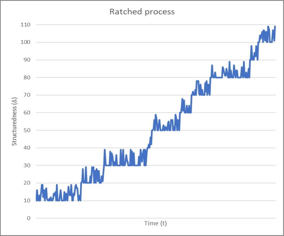

Then, due to the non-equilibrium of the system, the influx of energy from the outside forms some dissipative structures. Most of these dissipative structures disappear due to fluctuations of energy flow, but one of them eventually reaches the first threshold (in our case, 20) and becomes sufficiently structured to create a post-dissipative structure that will to be stable and will not disappear even if the influx of energy completely stops. After that, the structuredness of our system cannot be lower than this first threshold and will fluctuate (due to the emergence of new dissipative structures) only above this level until one of these dissipative structures achieves the second threshold, and so on.

As can be seen from Figure 4, the time intervals between the achievement of threshold values (“clicks” of the ratchet) can vary greatly, and sometimes they are quite long. The same could be said about the difference in structuredness between all adjacent thresholds. Although in Figure 4 they are all equal to 10 and equal to the initial structuredness, this was done only to clarify the ratchet process. In fact, all these quantities are different and can vary widely. In particular, the time intervals between thresholds in the real systems can be very large, especially when new dissipative structures emerge rarely.

This situation is typical for chemical evolution, since the appearance of a new, previously non-existent chemical compound as a product of an endothermic chemical reaction, occurred rarely. At the same time, the appearance of the subsequent post-dissipative structural elements, i.e., the new chemical compounds, did not depend on its “benefit” for the subsequent ratchet process. Accordingly, the structure genesis during chemical evolution, not only developed slowly, but its rate remained on average the same, without long-term decelerations or accelerations.

The emergence of life radically changed the situation. From the very beginning, living systems were encapsulated and separated from the environment by membranes ²⁶, which are also a kind of post-dissipative structures. As a result, each such encapsulated protocell had its own ratchet process, which created its own set of post-dissipative structural elements. Some of such sets were beneficial for the subsequent ratchet process while the others were not. These latter were eliminated by natural selection, because they did not create new diverse post-dissipative structural elements quickly enough and, thus, slowed down the evolution. In other words, the natural selection has turned the random and slow structure genesis of physicochemical systems into a directed and much faster biological evolution process.

Using metaphor, the ratchet process in inanimate systems can be compared to lifting weight, if you accidentally push the handle of the winch in opposite directions. In such a situation, only the ratchet mechanism provides a progressive, albeit slow movement of the weight upwards. In animate systems, on the other hand, the winch handle, due to natural selection, is pushing only in one direction, and the ratchet process becomes non random and accelerates sharply.

It is important to emphasize that the role of the ratchet, which is played by post-dissipative structural elements, is important, from the point of view of structuredness, only for one of the two possible directions of the structure genesis, namely, from chaos to maximum structuredness Δ. Another direction - from order to maximum structuredness - although it also forms post-dissipative structures, they, as mentioned above, do not generate ratchet processes. This happens because such post-dissipative structures are macro- and not microsystems and, accordingly, gradually disappear due to dissipation and degradation, i.e., their lifetime is limited. But structure genesis along this direction does not in fact need them, because it is collinear to the direction of general complification and, therefore, occurs by itself in accordance with the general law of complification.

It cannot be excluded that the emergence of life was in fact the result of precisely this direction of structure genesis. About 50 years ago Mikhail Kamshilov ²⁷ suggested principally new idea of ​​emergence of life. According Kamshivov, the life arose in a form of a whole biosphere as a complex system of geochemical cycles, which was subsequently divided into ecosystems and organisms. Later, Eric Smith and Harold J. Morowitz ²⁸ significantly developed this idea, enriching it with modern biogeochemical data. If so, then the top-down structure genesis determined the evolution on Earth, at least at that time, i.e., about 4 billion years ago. I am rather inclined to think that the process went from both top to bottom and bottom to top, and although one or the other direction probably dominated at different stages of evolution, only movement in both directions could lead to the emergence of life and its further structuredness.

Summing up this section, I would like to emphasize that, although there are two ways to increase the structuredness: “from order” and “from chaos”, only the latter requires some energy. At the same time, the first method is less common, since the ordered states of any system are the exception rather than the rule.

The more common structure genesis from chaos includes two phases. The first of these is the appearance of stable structures. They occur almost simultaneously with the formation of the systems themselves, does not require an influx of energy and are determined by one or another law of nature. On the contrary, this is usually accompanied by some release of energy, since the energy level of a stable state is lower than that of an unstable one. But after the appearance of stable structures, structure genesis enters the second phase, based on the appearance of dissipative structures. These structures require an influx of energy and can form post-dissipative, which do not require energy for their existence, but cannot appear without energy expenditure.

Such post-dissipative structures that have arisen at the micro level can exist as well as stable ones for an unlimited time. This property of post-dissipative structural elements ensures their accumulation as a result of the ratchet process. The ratchet process allows systems with dissipative and post-dissipative structures to develop in the direction of maximum structuredness, despite the fact that this is opposite to the direction of maximizing algorithmic complexity, determined by the general law of complification. This mechanism explains why the maximum of algorithmic complexity, information, and entropy (in other words, chaos) is unattainable in conditions of a permanent influx of energy, which we, thanks to the Sun and the internal heat of the Earth, have on our marvelous planet.

I am deeply grateful to Richard Gordon, Sergey Titov and Alexey Sharov for a very useful discussion of the ideas set forth in this article and thank my daughter Katerina Lomis and my friends Matya and Vladimir Karpov for their help in preparing this manuscript.

References

- 1.G E Mikhailovsky, A P Levich. (2015) Entropy, information and complexity or which aims the arrow of time?Entropy,17. [CrossRef] 4863-4890.
- 2.Thomson W. (1852) On a Universal Tendency in Nature to the Dissipation of. [CrossRef] , Mechanical Energy.Philos. Mag 4, 304-306.
- 3.J D Bowman, Rogers A E E, R A Monsalve, T J Mozdzen, Mahesh N. (2018) An absorption profile centred at 78 megahertz in the sky-averaged spectrum.Nature, 555. [PubMed] 67-70.
- 4.G E Mikhailovsky. (2018) From Identity to Uniqueness: The Emergence of Increasingly. Higher Levels of Hierarchy in the Process of the Matter Evolution.Entropy,20 [CrossRef] 533-551.
- 5.M L Rosenzweig. (1995) Species Diversity in Space and Time, CambridgeUniversityPress. [SciRes] , New York, NY
- 7.Mouillot D, Lepretre A. (2000) Introduction of Relative Abundance Distribution (RAD) Indices, Estimated from the Rank-Frequency Diagrams (RFD), to Assess Changes. in Community Diversity.Environ. Monitoring and Assessment,63 [CrossRef] 279-295.
- 8.Oskin B, Writer S. (2014) Confirmed: Oldest Fragment of Early Earth is 4.4 Billion Years Old.LifeScience. [LifeSci]
- 9.R J Solomonoff. (1964) A Formal Theory of Inductive Inference. Part I and 2.Inf. Control,7[1–22][224–254] [PDF1] [PDF2]
- 10.A N Kolmogorov.Three Approaches to the Quantitative Definition. of Information.Probl. Inf.Transm.1965,1 1-7.
- 11.G J Chaitin. (1969) On the Length of Programs for Computing Finite Binary Sequences:. , Statistical Considerations.J. Assoc. Comput. Mach 16, 145-159.
- 12.M A Fuentes.. Complexity and the Emergence of Physical Properties.Entropy2014,16 [Cross Ref] 4489-4496.
- 13.C H Lineweaver. (2013) A Simple Treatment of Complexity: Cosmological Entropic Boundary Conditions on Increasing Complexity. InComplexity and the Arrow of Time. , Lineweaver, C.H., Davis, P.C.W., Ruse, M., Eds.; Cambridge University Press: Cambridge, UK 42-67.
- 14.C H Bennet. (1988) Logical Depth and Physical Complexity. InThe Universal Turing Machine: a Half-Century Survey. 2nd ed.; Herken, R., Ed.; , OxfordUniversityPress: Oxford, NY 227-257.
- 15.Antunes L, Fortnow L. (2009) . Sophistication Revisited.Theory of Computing Systems,45 [Cross Ref] 150-161.
- 16.Rissanen J. (1986) . Stochastic Complexity and Modelling.The Annals of Statistics,14 [Sci Res] 1080-1100.
- 17.Kumar U, Kumar V, J N Kapur. (1986) . [CrossRef] , Normalized Measures of Entropy.Int. Jour. of General Systems 12, 55-69.
- 18.Gorelick R, S M Bertram, P R Killeen, J H Fewell. (2004) . [CrossRef] , Notes and Comments: Normalized Mutual Entropy in Biology: Quantifying Division of Labor.The American Naturalist 164, 677-682.
- 19.C E Shannon. (1948) . The Mathematical Theory of Communication.The Bell System Technical Journal27[379–423][623–656] .
- 20.Banaty B. (2019) A Taste of Systemics. Types of Systems. [Available online] (accessed on 04April)
- 22.I Glansdorff P Prigogine. (1971) Thermodynamic Theory of Structure, Stability and Fluctuations, JohnWileySons. , New York, NY
- 23.Schneider E D, Kay J J. (1995) Order from Disorder: The Thermodynamics of Complexity in Biology, InWhat is Life: The Next Fifty Years. Reflections on the Future of Biology, Murphy. , M.P.,LukeA.J,O'Neill,L.A.J.,Eds.,Cambridge UniversityPress:Cambridge,UK 161-172.
- 24.Kondepudi D, Petrosky T, J A Pojman. (2017) Dissipative structures and irreversibility in nature:. Celebrating 100th birth anniversary of Ilya Prigogine (1917–2003).Chaos [CrossRef] 27-104501.
- 25.Goldbeter A. (2018) Dissipative structures in biological systems: bistability, oscillations, spatial patterns and waves.Phil. [CrossRef] , Trans. R. Soc.A,376: 2124.